-
-
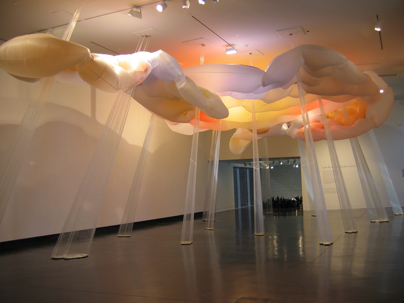
Lucky Storm, 2004
-
View Picture
-
-
-
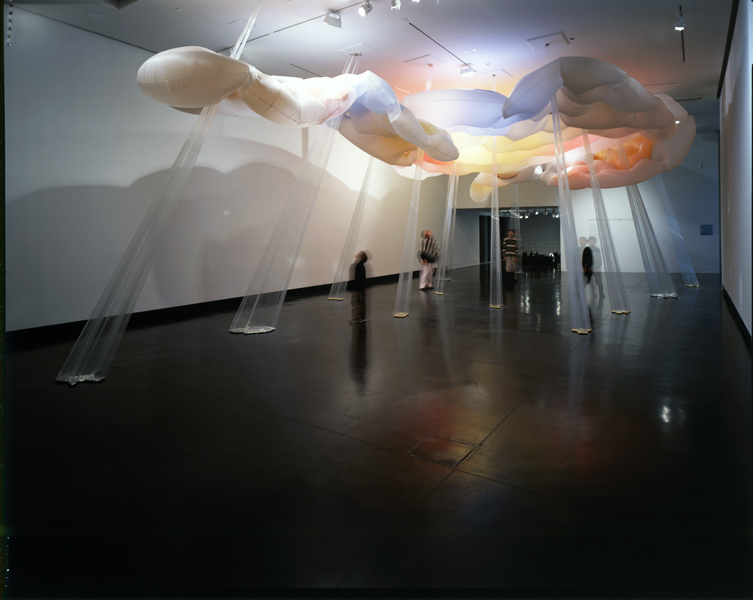
Lucky Storm, 2004
-
View Picture
-
-
-
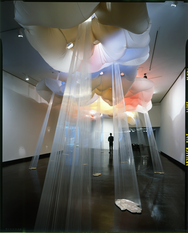
Lucky Storm, 2004
-
View Picture
-
-

-
Outer Limit, 2005
-
View Picture
-
-
-
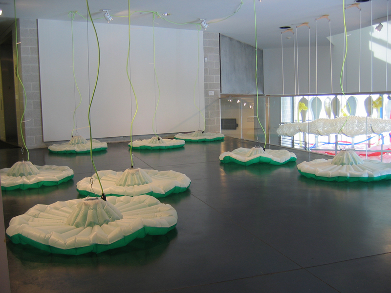
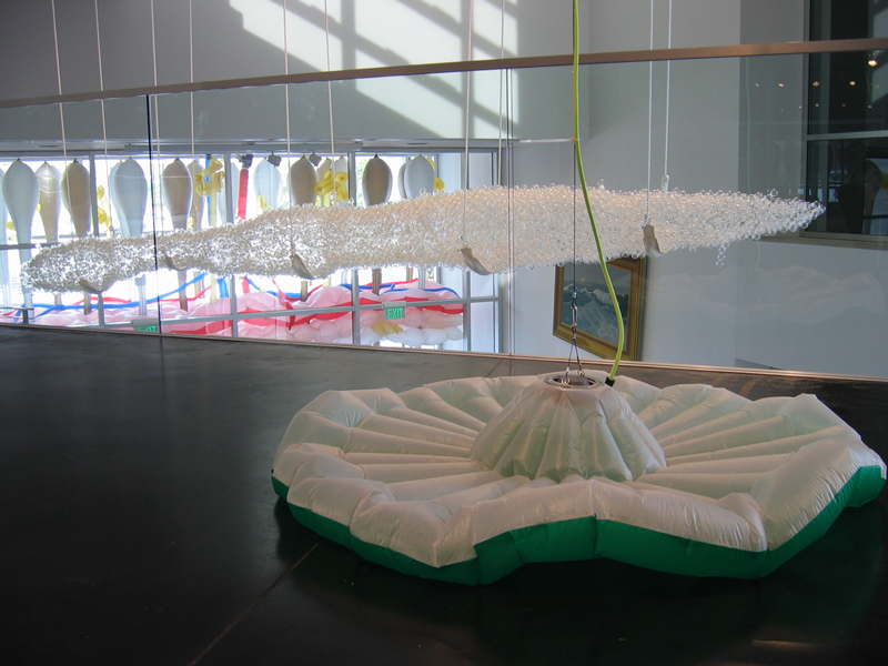
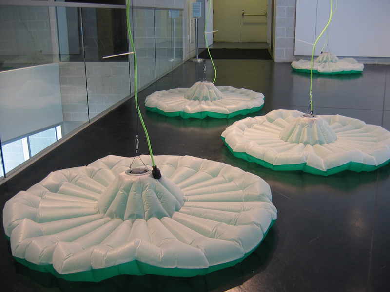
Pleasure Grounds, 2005
-
View Picture
-
-
-
Pleasure Grounds, 2005
-
View Picture
-
-
-
Pleasure Grounds, 2005
-
View Picture
-
-
-
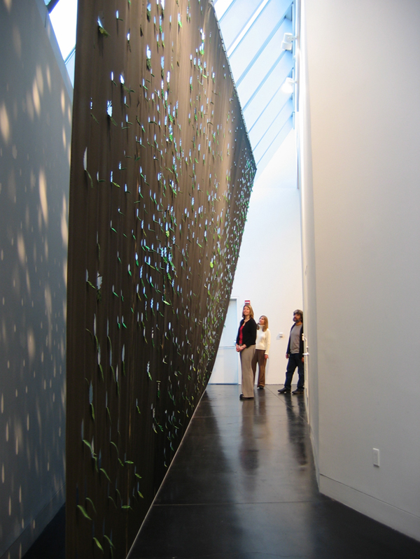
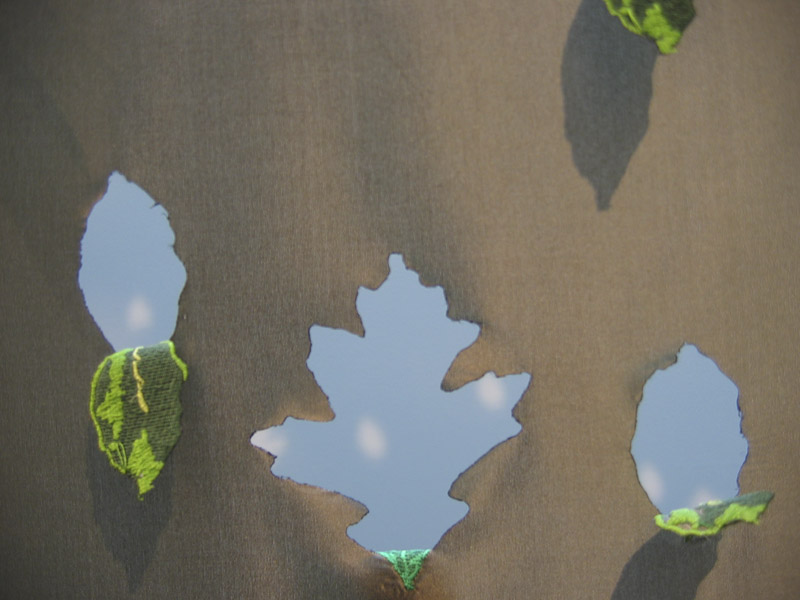
Trim, 2005
-
View Picture
-
-
-
Trim, 2005
-
View Picture
-
-
-
Trim, 2005
-
View Picture
-
-
-
CI: Star Swarm, 2005
-
View Picture
-
-
-
CI: Star Swarm, 2005
-
View Picture
-
Lee Boroson- Outer Limit, The Tang Teaching Museum and Art Gallery, Skidmore College, Saratoga Springs, NY 2005
The eighth installment of the Opener series features seven large-scale works by Brooklyn- based artist Lee Boroson. Since 1995, Boroson has been known for his room-filling inflated sculptures. These colorful sewn-nylon enclosures find inspiration in many sources, from historic garden design to the architectural details of their sites. Integument, a buoyant piece installed in the Tang’s vestibule, compares an often-overlooked section of the building to a layer of skin. Pleasure Grounds, an inflated environment of lily pad-like forms, and Dewpoint, an accumulation of thousands of tiny glass spheres that form a hanging cloud, are amalgams of the manufactured and the magical. Other new works grow from the microscopic to the macrocosmic, such as a meticulously manipulated photograph that attempts to picture the visible night sky with all of its black space removed.
“Outer Limit”, 2005, dimensions variable, wood, paint, metal flake. Installed at Tang Museum. Based on architectural forms derived from similar representations in Hudson River School painting practice where looming architectural structures are presented as a sort of garden folly. (Part of exhibition: Lee Boroson, Outer Limit, Tang Museum, Saratoga Springs, NY)
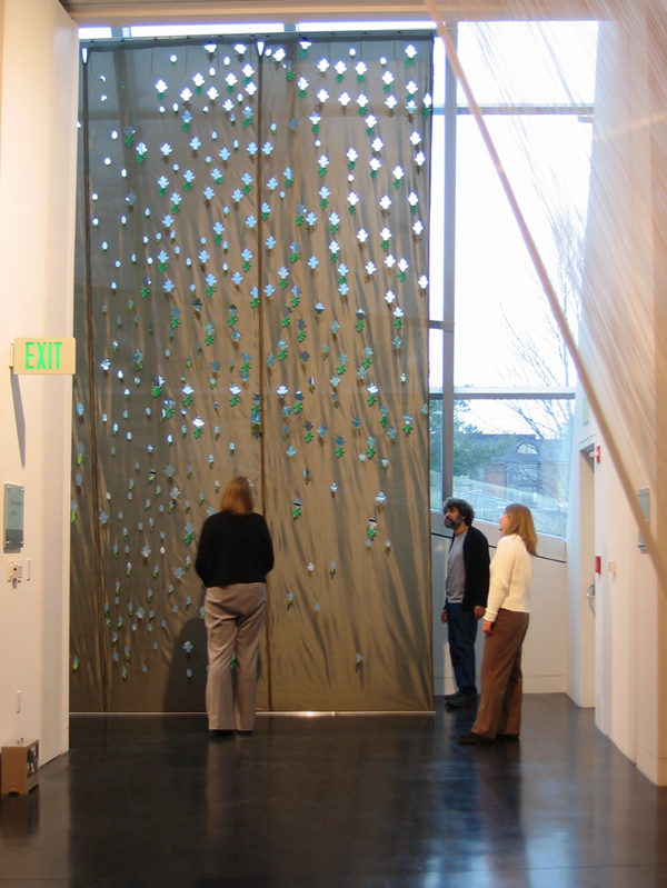
“Trim”, 2005, 45’x17’x3’, polyester fabric, embroidery. Installed at the Tang Museum. (Part of exhibition: Lee Boroson, Outer Limit, Tang Museum, Saratoga Springs, NY)
“Lucky Storm”, 2004, Dimensions vary. Nylon, monofilament, stainless steel, hardware, blower. Seven “crepuscular rays” (an atmospheric optical phenomenon) appear out of an ominous “storm cloud”. This is one part of a three-part installation that alters the spaces of the gallery with elements derived from American romantic landscape painting, especially the pre-photographic interpretation of landscape found in Thomas Cole’s paintings and those of the Hudson River School painters. Nature is frequently presented as a fantastic amalgam of real detail and impossible phenomena, not observed but reinvented for the purpose of allegorical narrative.
The rays are in the shapes of lucky and superstitious charms laser cut out of stainless steel, then strung like a harp with fishing line. The cloud form is made of nylon fabric, supported pneumatically. The coloration is an effect caused by colored material sewed into the translucent fabric.
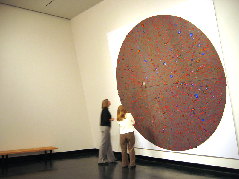
“CI: Star Swarm”, 2005, 12’ x 12’, digital c-print, mounted on aluminum under plexiglass
Celestial Incorporation – Technical Background on data and processing
The Data
The images come from the Sloan Digital Sky Survey[1] (SDSS) , a multi-year project that aims to image about one-fifth of the sky in 5 colors and obtain spectra of about one million galaxies and 100,000 quasars. The survey began its observations in 1998 and now, at the end of 2004, they are almost complete. Observations are made with a 2.5 meter diameter telescope at Apache Point Observatory, in southern New Mexico. The images are obtained using a custom camera that uses thirty separate 4 megapixel CCD detectors, with 6 dedicated to each of the 5 color bands. The instrument is used in a TDI (Time Delay Integrate) mode, in which the telescope is fixed in position, and the sky drifts past (because of the rotation of the earth). The data comes out as a long swath on the sky in each of the five colors, which are slightly offset in time. The effective integration time per color is about 55 seconds, and the “limiting magnitude” for the data is between 19th and 20th magnitude[2]. SDSS maintains an excellent web site (www.sdss.org) on which can be found many details about the instrument, the software, the survey operations, and the data. The data are made publicly available over the internet through a data access tool called SkyServer[3] (http://cas.sdss.org/dr3/en/).
At the time that we began the Celestial Incorporation project, Data Release 2 (DR2) of the SDSS had just been made available. DR2 included about 3300 square degrees[4] (approximately 40% of the 8500 square degrees that SDSS will eventually cover). One of the ways in which the SDSS makes data available is as jpeg files with formats up to 2048 X 2048 pixels. At the nominal spatial scale of the camera (0.396 arcseconds/pixel), this maximum size corresponds to an area of about 0.05 square degrees. Thus, there are about 20 of these files per square degree. For our large Celestial Incorporation image, we downloaded 2000 square degrees – about 40,000 separate jpeg files – of SDSS DR2 data.
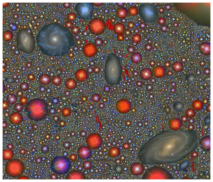
The jpegs are made using filters termed g (for green), r (for red), and i (for infrared) – and these three separate monochromatic images are registered and combined into a single color image. The colors are approximate or subjective, in that g,r, and i are converted into blue, green, and red, and also because the eye’s color sensitivity is diminished or altered at faint light levels (don’t most stars look white?).
The Processing
The processing of the Celestial Incorporation data was done on a PC with a 2.4 GHz Pentium-4 CPU and 1 Gigabyte of physical memory. The operating system was Red Hat 9 Linux. The programs were written in the C language, but also used system calls to lynx, a text-based web browser, and ImageMagick, a suite of applications for manipulating images. The data download took about 40 hours (over a cable modem) and the processing required about 100 hours (of computer time) stretched over approximately a month. An additional 100 hours was spent during this time looking at intermediate images, manipulating the input data, and tweaking the programs. A number of smaller datasets were processed first. A fundamental limit was the memory limit of 2 Gigabytes imposed by the 32-bit architecture of the computer. Since each pixel in the final image requires 3 bytes, a square image greater than about 25,000 pixels on the edge would require more than 2 Gigabytes of memory. There are a number of ways around this limitation; we chose to divide the final image into quadrants and process them separately until the final stages (which were done using Adobe Photoshop, which apparently has its own memory management scheme, and splits files into pieces that it can swap on and off a large temporary disk file).
The basic program works as follows: The input files, each 2048X2048 pixels or about 0.05 square degrees, were ordered by distance from the nominal center of the output image, the position in the sky xxx hours right ascension, yyy degrees declination. The program processed the innermost ones first and the outermost ones last. For each input file, the program found all the objects brighter than a given limit that corresponded to a magnitude of zzz. As each object was found, its edges were determined and a “postage stamp” of that object was extracted. A second pass attempted to clean up artifacts. The objects from a given file were ordered by their distance from the central position of the output image. For each object, its position angle relative to the central position was determined. It was then nestled into the output image at an angle close to its actual one, but in a way that tried to squeeze it in as far as possible. A small amount of overlap on top of existing images was allowed. Objects that crossed the boundaries of input files were discarded. The output cluster was built up until its radius reached a limit – about 10,000 pixels. This represented the maximum size image that could be processed.
The image was then split into four quadrants, and each of these quadrants became the inner quadrant of a new file. These new files were then processed with a similar program that built up the cluster from the inner corner rather than the center of the output image. Files were fed in until the cluster reached a size of about 21,000 pixels in radius from the inner corner. Because the program did not allow objects to be placed such that they extended over the edge of the file, there was a small gap between the objects and edge. When the quadrants were assembled into a single image, these gaps were filled in by hand.
Some interesting aspects:
Number of objects – Although the number of objects per square degree varies over the sky, there were approximately 300 objects extracted per input file. So, for 40,000 input files processed, the final image contains about 12 million separate objects. Note that the region covered by SDSS excludes the galactic plane (the disk of our galaxy, the Milky Way), where the number of stars per square degree is much higher.
Faintest objects – The faintest objects extracted by the program are approximately magnitude 20, which is about 14 magnitudes (or a factor of 400,000) fainter than the faintest stars that one can see with the unaided eye in a dark sky. A few thousand stars are magnitude 6 or brighter over the whole sky. The objects in the final output image are a mix of stars and galaxies. The stars are all in our galaxy. At this faintest brightness, the number of stars per square degree (which falls off with decreasing brightness) is about equal to the number of galaxies per square degree (which rises with decreasing brightness).
Size of star images – If you could see the stars without the blurring effects of the earth’s atmosphere, they would be much smaller in size than they appear in the images from ground-based telescopes. For example, a star of magnitude 11 is a pretty bright star as seen in the SDSS images. It has quite obvious diffraction spikes (the cross of lines that can be seen going out from the brighter stars – caused by diffraction of light around the structure that holds the secondary mirror of the telescope in place), and the program finds that such a star “goes out” about 10 pixels from its center. This corresponds to a diameter of about 8 arcseconds. If this star were a star like the sun (an average star), it would be at a distance of about 160 parsecs, and its apparent size would be 60 micro-arcseconds or 1.5 ten-thousandths of a pixel.
Galaxies distances and sizes – The galaxies are much bigger (typically 10,000 parsecs in diameter) and much further away. Their images are also blurred by the atmosphere but the result of this is primarily to make them less distinct rather than to make them appear larger in size. A typical galaxy is made up of a billion or so stars ranging from a few that are thousands of times brighter than the sun, to many that are one-tenth as bright as the sun.
Extending project – Ultimately, SDSS will cover about 9000 square degrees. If we process those data in the same way, it will produce a “cluster” that is about 25 feet in diameter. This is still only about one-fifth of the visible sky. It still excludes the plane of our galaxy and most of the region south of that plane, much of which is only visible from the southern hemisphere.
[1] The Sloan Digital Sky Survey (SDSS) is a joint project of The University of Chicago, Fermilab, the Institute for Advanced Study, the Japan Participation Group, The Johns Hopkins University, The Korean Scientist Group (KSG), the Los Alamos National Laboratory, the Max-Planck-Institute for Astronomy (MPIA), the Max-Planck-Institute for Astrophysics (MPA), New Mexico State University, University of Pittsburgh, Princeton University, the United States Naval Observatory, and the University of Washington.
Funding for the project has been provided by the Alfred P. Sloan Foundation, the Participating Institutions, the National Aeronautics and Space Administration, the National Science Foundation, the U.S. Department of Energy, the Japanese Monbukagakusho, and the Max Planck Society.
[2] Astronomers use the “magnitude” system to indicate the apparent brightness of objects in the sky. Objects with larger magnitudes are fainter, with a step of one magnitude corresponding to a brightness ratio of about 2.5 (the one-fifth root of 100, actually). Although the exact number depends on the color in which it is measured, the brightest star, Sirius, has a brightness of about –1.5 magnitude and the faintest stars that you can see at a dark site with just your eyes are about 6th magnitude. The faintest stars studied with the largest telescopes are in the magnitude range 28-30.
[3] The SDSS Data Releases are the product of efforts by many individuals supported by many institutions. The Johns Hopkins University has had a lead role in the design and implementation of the SDSS database and the associated query tools. The Space Telescope Science Institute has developed some of the web interfaces, coordinated the assembly of user documentation for the Early Data Release. Fermilab has provided key support for the data servers, system testing, and project management.
The Microsoft Bay Area Research Center helped develop the SkyServer and its interface, and Microsoft Research has contributed computing hardware and software for the SkyServer.
The following is an incomplete list of the individuals who have contributed to the SkyServer.
Development: Tom Barclay, Bill Boroski, Karen Brown, Tamas Budavari, Sam Carliles, Roy Gal, Jim Gray, Vivek Haridas, Sebastian Jester, Steve Kent, Peter Kunszt, Rich Kron, Steve Landy, Blair Lanier, Nolan Li, Tanu Malik, Maria Nieto-Santisteban, Tim Olson, Wil O’Mullane, Adrian Pope, Jordan Raddick, Asta Roseway, Robert Sparks, Chris Stoughton, Mark SubbaRao, Don Slutz, Alex Szalay, Tamas Szalay, Ani Thakar, Jan Vandenberg, Curtis Wong, Wei Zheng.
Translation: Sadanori Okamura, Naoki Yasuda, Matthias Bartelmann
Testing: Rosa Gonzalez, Kausar Yasmin, Karl Glazebrook, Robert Lupton
[4] The celestial sphere contains 41,253 square degrees. For reference, the sun or full moon has a diameter of about 0.5 square degrees, or an area of about 0.2 square degrees.

